First set up Zorn/Bascet according to the install instructions, e.g.:
library(Zorn)
bascetRunner.default <- LocalRunner()
bascetInstance.default <- getBascetBinary()
Bascet assumes that you have a “workspace” where all processed files will land. We call this the bascetRoot. Set it up first:
bascetRoot <- file.path("/home/yours/an_empty_workdirectory")The first data processing step is to read the raw FASTQ files and identify which read belongs to which cell. Zorn can automatically figure out which files to use for what:
rawmeta <- DetectRawFileMeta("/home/yours/directory_with_raw_fastq")⚠️ Input FASTQs must be bgzipped (
.fastq.gzwritten bybgzip), not produced by plaingzip. Bascet relies on the block structure of BGZF to read the files in parallel. FASTQs straight off an Illumina sequencer are already bgzipped, but if you have re-compressed files (or downloaded.gzfiles from elsewhere) you may need to recompress withbgzipfirst. Decompress to a real file first, then bgzip it:gunzip reads.fastq.gz # produces reads.fastq bgzip reads.fastq # produces reads.fastq.gz (bgzipped)⚠️ Do not pipe into
bgzip(e.g.zcat reads.fastq.gz | bgzip > ...). It silently produces a file that looks valid but is not correctly block-compressed, and Bascet will fail to read it in parallel. Always runbgzipon a real file.
Depending on your input data, rawmeta might look like this:
| prefix | r1 | r2 | dir |
|---|---|---|---|
| UDI_Plate_WT_29 | UDI_Plate_WT_29_S43_L007_R1_001.fastq.gz | UDI_Plate_WT_29_S43_L007_R2_001.fastq.gz | /home/m/mahogny/mystore/dataset/250611/fastq |
| UDI_Plate_WT_29 | UDI_Plate_WT_29_S43_L008_R1_001.fastq.gz | UDI_Plate_WT_29_S43_L008_R2_001.fastq.gz | /home/m/mahogny/mystore/dataset/250611/fastq |
| UDI_Plate_WT_30 | UDI_Plate_WT_30_S44_L007_R1_001.fastq.gz | UDI_Plate_WT_30_S44_L007_R2_001.fastq.gz | /home/m/mahogny/mystore/dataset/250611/fastq |
| UDI_Plate_WT_30 | UDI_Plate_WT_30_S44_L008_R1_001.fastq.gz | UDI_Plate_WT_30_S44_L008_R2_001.fastq.gz | /home/m/mahogny/mystore/dataset/250611/fastq |
Prefix is the name of the library, of which there are two here. Note the paired input FASTQ files R1 and R2. Zorn has here detected that the libraries were sequenced on two separate lanes; by using the same prefix, these will be merged during the later sharding stage. Keeping input files from different lanes separate enables each FASTQ file to be processed on a separate computer and can thus be advantageous if you have large amounts of data.
If you have files that are awkwardly named for some reason, simply produce a data frame with the columns above, and provide as input for the next stage.
You can now parse the reads the figure out which cell they belong to, and any UMI information. The only thing you additionally need to specify is what type of data you have, where “atrandi-wgs” is for the Atrandi SPC-based MDA protocol for WGS.
⚠️ Note that Bascet performs trimming of reads during the Debarcode stage. This includes: - For RNA-seq: PolyA trimming and trimming at adapters - For Atrandi WGS: A specialized algorithm to detect overlap and remove adapters accordingly Regular users should thus not need to worry about this
BascetDebarcode(
    bascetRoot,
    rawmeta,
    chemistry="atrandi-wgs"
)
Chemistries supported right now are: - atrandi-wgs —
Atrandi SPC-based MDA protocol for WGS - atrandi-wgslr —
Atrandi SPC-based MDA protocol for WGS, long-read -
atrandi-rnaseq — Atrandi SPC-based protocol for RNA-seq -
parse-bio — Parse Biosciences RNA-seq - tenx —
10x Genomics (3’/5’ v2/v3/v3.1/v4, multiome)
After debarcoding, you now need to (1) merge files belong to the same library, and (2) remove reads belonging to empty droplets. Furthermore, at this step you can also decide to split the cells across multiple “shards”, enabling parallel processing the data in later steps. This done in two steps, in which you first set up a “plan”. This is done using the following command:
debstat <- PrepareSharding(
  bascetRoot,
  inputName="debarcoded",
  minQuantile=0.95                         #Lower number keeps more cells; do more thorough filtering later
)
Before you proceed, you should perform a kneeplot analysis to see which cells you keep:
DebarcodedKneePlot(
debstat,
filename = "kneeplot.pdf" #optional
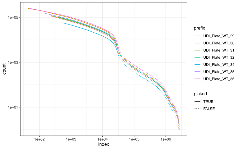
)This is just a histogram of reads per barcode. (downsampling for speed causes cells of low indices to not be shown, worry not!) The diagram however tells you - how many cells you have - how much free-floating RNA/DNA you have in your background (empty droplets/SPCs) - how distinct cells are from background
An example kneeplot for Parse biosciences RNA-seq data is shown below. You want to include slightly more cells than the knee indicates. For Atrandi microbial WGS data, knee plots cannot be trusted, and you may want a fair bit more to account for lysis differences (see our manuscript). Including too many cells will slow down later steps but you can reduce the number of cells at any point. Adjust the cutoff using the previously set minQuantile parameter.
Once you have a plan you are happy with, you can proceed with shardification. At this step you can also choose to create multiple shards. This is only relevant if you wish to parallelize the workflow using SLURM, as the number of shards decides how many nodes you can use in parallel. If you run everything on your own computer then we advise only creating one shard, as there is no benefit to having multiple and it is more likely to cause mistakes.
BascetShardify(
  debstat,
  numOutputShards = 10 #Shards per library; increase to spread the workload over more computers
)
Onward
If you make it here then you have passed one of the heaviest and most critical steps in the workflow!
How you proceed depends on your use case. If you are doing single-cell metagenomics of a sample of unknown composition then we recommend the KRAKEN2 workflow next.
Advanced users may wish to get FASTQ files as input for other tools. (SLURM-compatible step)